1. BigSim Parallel Simulator
Contents
1.1. Introduction
Parallel machines with an extremely large number of processors are now being designed and built. For example, the BlueGene/L (BG/L) machine built by IBM has 64,000 dual-processor nodes with 360 teraflops of peak performance. Another more radical design from IBM, code-named Cyclops (BlueGene/C), had over one million floating point units, fed by 8 million instructions streams supported by individual thread units, targeting 1 petaflops of peak performance.
It is important that one can study the programming issues and performance of parallel applications on such machines even before the machine is built. Thus, we have developed a parallel simulator - BigSim, to facilitate this research.
Since our research was initiated by the BlueGene/C project, in previous editions of this manual we also called our simulator as Blue Gene Simulator. Our simulator is capable of simulating a broad class of “Massively Parallel Processors-In-Memory”, or MPPIM machines.
1.1.1. Simulator system components
Our simulator system includes these components:
- a parallel emulator which emulates a low level machine API targeting an architecture like BlueGene;
- a message driven programming language (Charm++) running on top of the emulator;
- the Adaptive MPI (an implementation of MPI on top of Charm++) environment;
- a parallel post-mortem mode simulator for performance prediction, including network simulation.
1.1.2. History
The first version of the BlueGene emulator was written in Charm++, a parallel object language, in fall 2001. The second version of the BlueGene emulator was completely rewritten on top of Converse instead of Charm++ in spring 2002. While the API supported by the original emulator remains almost the same, many new features were added. The new emulator was implemented on a portable low layer communication library - Converse, in order to achieve better performance by avoiding the cross layer overhead.
Charm++ was ported to the emulator in 2002, providing the first parallel language model on top of the emulator.
A performance simulation capability was added to the emulator in spring 2003. The new simulator was renamed to BigSim at the same time. During the same year, we developed a POSE-based postmortem mode network simulator called BigNetSim. In fall 2006, we renamed BigNetSim as simply BigSim simulator.
In the following sections, we will first describe how to download and compile the BigSim system (Section 1.2). Section 1.3 describes the BigSim Emulator and the low level machine API in detail.
1.2. BigSim Emulator Installation and Usage
1.2.1. Installing Charm++ and BigSim
The BigSim Emulator is distributed as part of the Charm++ standard distribution. One needs to download Charm++ and compile the BigSim Simulator. This process should begin with downloading Charm++ from the website: http://charm.cs.uiuc.edu.
Please refer to “Charm++ Installation and Usage Manual” and also the file README in the source code for detailed instructions on how to compile Charm++. In short, the “build” script is the main tool for compiling Charm++. One needs to provide target and platform selections:
$ ./build <target> <platform> [options ...] [charmc-options ...]
For example, to compile on a 64-bit Linux machine, one would type:
$ ./build charm++ netlrts-linux-x86_64 -O2
which builds essential Charm++ kernel using UDP sockets as the communication method; alternatively, it is possible to build the Charm++ kernel on MPI using:
$ ./build charm++ mpi-linux-x86_64 -O2
For other platforms, netlrts-linux-x86_64 should be replaced by whatever platform is being used. See the charm/README file for a complete list of supported platforms.
1.2.1.1. Building Only the BigSim Emulator
The BigSim Emulator is implemented on top of Converse in Charm++. To compile the BigSim Emulator, one can compile Emulator libraries directly on top of normal Charm++ using “bgampi” as the compilation target, like
$ ./build bgampi netlrts-linux-x86_64 -O2
With Emulator libraries, one can write BigSim applications using its low level machine API (defined in 1.3).
1.2.1.2. Building Charm++ or AMPI on the BigSim Emulator
In order to build Charm++ or AMPI on top of BigSim Emulator (which itself is implemented on top of Converse), a special build option “bigemulator” needs to be specified:
$ ./build bgampi netlrts-linux-x86_64 bigemulator -O2
The “bgampi” option is the compilation target that tells “build” to compile BigSim Emulator libraries in addition to Charm++ kernel libraries. The “bigemulator” option is a build option to platform “netlrts-linux”, which tells “build” to build Charm++ on top of the BigSim Emulator.
The above “build” command creates a directory named “netlrts-linux-x86_64-bigemulator” under charm, which contains all the header files and libraries needed for compiling a user application. With this version of Charm++, one can run normal Charm++ and AMPI application on top of the emulator (in a virtualized environment).
1.2.2. Compiling BigSim Applications
Charm++ provides a compiler script charmc to compile all programs.
As will be described in this subsection, there are three methods to
write a BigSim application: (a) using the low level machine API, (b)
using Charm++ or (c) using AMPI. Methods (b) and (c) are essentially
used to obtain traces from the BigSim Emulator, such that one can use
those traces in a post-mortem simulation as explained in
Section 2.1.
1.2.2.1. Writing a BigSim application using low level machine API
The original goal of the low level machine API was to mimic the BlueGene/C low level programming API. It is defined in section 1.3. Writing a program in the low level machine API, one just needs to link Charm++’s BigSim emulator libraries, which provide the emulation of the machine API using Converse as the communication layer.
In order to link against the BigSim library, one must specify
-language bigsim as an argument to the charmc command, for
example:
$ charmc -o hello hello.C -language bigsim
Sample applications in low level machine API can be found in the directory charm/examples/bigsim/emulator/.
1.2.2.2. Writing a BigSim application in Charm++
One can write a normal Charm++ application which can automatically run on the BigSim Emulator after compilation. Charm++ implements an object-based message-driven execution model. In Charm++ applications, there are collections of C++ objects, which communicate by remotely invoking methods on other objects via messages.
To compile a program written in Charm++ on the BigSim Emulator, one
specifies -language charm++ as an argument to the charmc
command:
$ charmc -o hello hello.C -language charm++
This will link both Charm++ runtime libraries and BigSim Emulator libraries.
Sample applications in Charm++ can be found in the directory charm/examples/bigsim, specifically charm/examples/bigsim/emulator/littleMD.
1.2.2.3. Writing a BigSim application in MPI
One can also write an MPI application for the BigSim Emulator. Adaptive MPI, or AMPI, is implemented on top of Charm++, supporting dynamic load balancing and multithreading for MPI applications. Those are based on the user-level migrating threads and load balancing capabilities provided by the Charm++ framework. This allows legacy MPI programs to run on top of BigSim Charm++ and take advantage of the Charm++’s virtualization and adaptive load balancing capability.
Currently, AMPI implements most features in the MPI version 1.0, with a few extensions for migrating threads and asynchronous reduction.
To compile an AMPI application for the BigSim Emulator, one needs to
link against the AMPI library as well as the BigSim Charm++ runtime
libraries by specifying -language ampi as an argument to the
charmc command:
$ charmc -o hello hello.C -language ampi
Sample applications in AMPI can be found in the directory
charm/examples/ampi. See also charm/benchmarks/ampi/pingpong.
1.2.3. Running a BigSim Application
To run a parallel BigSim application, Charm++ provides a utility program
called charmrun that starts the parallel execution. For detailed
description on how to run a Charm++ application, refer to the file
charm/README in the source code distribution.
To run a BigSim application, one needs to specify the following
parameters to charmrun to define the simulated machine size:
+vp: define the number of processors of the hypothetical (future) system+x,+yand+z: optionally define the size of the machine in three dimensions, these define the number of nodes along each dimension of the machine (assuming a torus/mesh topology);+wthand+cth: For one node, these two parameters define the number of worker processors (+wth) and the number of communication processors (+cth).+bgwalltime: used only in simulation mode, when specified, use wallclock measurement of the time taken on the simulating machine to estimate the time it takes to run on the target machine.+bgcounter: used only in simulation mode, when specified, use the performance counter to estimate the time on target machine. This is currently only supported when perfex is installed, like Origin2000.+bglog: generate BigSim trace log files, which can be used with BigNetSim.+bgcorrect: starts the simulation mode to predict performance. Without this option, a program simply runs on the emulator without doing any performance prediction. Note: this option is obsolete, and no longer maintained, use +bglog to generate trace logs, and use BigNetSim for performance prediction.
For example, to simulate a parallel machine of size 64K as 40x40x40, with one worker processor and one communication processor on each node, and use 100 real processors to run the simulation, the command to be issued should be:
$ ./charmrun +p100 ./hello +x40 +y40 +z40 +cth1 +wth1
To run an AMPI program, one may also want to specify the number of
virtual processors to run the MPI code by using +vp. As an example,
$ ./charmrun +p100 ./hello +x40 +y40 +z40 +cth1 +wth1 +vp 128000
starts the simulation of a machine of size 40x40x40 with one worker
processor in each node, running 128000 MPI tasks (2 MPI tasks on each
node), using 100 real processors to run the simulation. In this case,
MPI_Comm_size() returns 128000 for MPI_COMM_WORLD. If the
+vp option is not specified, the number of virtual processors will
be equal to the number of worker processors of the simulated machine, in
this case 64000.
1.3. BigSim Emulator
The BigSim emulator environment is designed with the following objectives:
- To support a realistic BigSim API on existing parallel machines
- To obtain first-order performance estimates of algorithms
- To facilitate implementations of alternate programming models for Blue Gene
The machine supported by the emulator consists of three-dimensional grid of 1-chip nodes. The user may specify the size of the machine along each dimension (e.g. 34x34x36). The chip supports \(k\) threads (e.g. 200), each with its own integer unit. The proximity of the integer unit with individual memory modules within a chip is not currently modeled.
The API supported by the emulator can be broken down into several components:
- Low-level API for chip-to-chip communication
- Mid-level API that supports local micro-tasking with a chip level scheduler with features such as: read-only variables, reductions, broadcasts, distributed tables, get/put operations
- Migratable objects with automatic load balancing support
Of these, the first two have been implemented. The simple time stamping algorithm, without error correction, has been implemented. More sophisticated timing algorithms, specifically aimed at error correction, and more sophisticated features (2, 3, and others), as well as libraries of commonly needed parallel operations are part of the proposed work for future.
The following sections define the appropriate parts of the API, with example programs and instructions for executing them.
1.3.1. BigSim Programming Environment
The basic philosophy of the BigSim Emulator is to hide intricate details of the simulated machine from the application developer. Thus, the application developer needs to provide initialization details and handler functions only and gets the result as though running on a real machine. Communication, Thread creation, Time Stamping, etc are done by the emulator.
1.3.1.1. BigSim API: Level 0
void addBgNodeInbuffer(bgMsg *msgPtr, int nodeID)
low-level primitive invoked by Blue Gene emulator to put the message to the inbuffer queue of a node.
msgPtr - pointer to the message to be sent to target node;
nodeID - node ID of the target node, it is the serial number of a bluegene node in the emulator’s physical node.
void addBgThreadMessage(bgMsg *msgPtr, int threadID)
add a message to a thread’s affinity queue, these messages can be only executed by a specific thread indicated by threadID.
void addBgNodeMessage(bgMsg *msgPtr)
add a message to a node’s non-affinity queue, these messages can be executed by any thread in the node.
boolean checkReady()
invoked by communication thread to see if there is any unattended message in inBuffer.
bgMsg * getFullBuffer()
invoked by communication thread to retrieve the unattended message in inBuffer.
CmiHandler msgHandlerFunc(char *msg)
Handler function type that user can register to handle the message.
void sendPacket(int x, int y, int z, int msgSize,bgMsg *msg)
chip-to-chip communication function. It send a message to Node[x][y][z].
bgMsg is the message type with message envelope used internally.
1.3.1.2. Initialization API: Level 1a
All the functions defined in API Level 0 are used internally for the implementation of bluegene node communication and worker threads.
From this level, the functions defined are exposed to users to write bluegene programs on the emulator.
Considering that the emulator machine will emulate several Bluegene nodes on each physical node, the emulator program defines this function BgEmulatorInit(int argc, char **argv) to initialize each emulator node. In this function, user program can define the Bluegene machine size, number of communication/worker threads, and check the command line arguments.
The size of the simulated machine being emulated and the number of thread per node is determined either by the command line arguments or calling following functions:
void BgSetSize(int sx, int sy, int sz)
set Blue Gene Machine size;
void BgSetNumWorkThread(int num)
set number of worker threads per node;
void BgSetNumCommThread(int num)
set number of communication threads per node;
int BgRegisterHandler(BgHandler h)
register user message handler functions;
For each simulated node, the execution starts at BgNodeStart(int argc,
char **argv) called by the emulator, where application handlers can be
registered and computation is triggered by creating a task at required
nodes.
Similar to pthread’s thread specific data, each bluegene node has its own node specific data associated with it. To do this, the user needs to define its own node-specific variables encapsulated in a struct definition and register the pointer to the data with the emulator by following function:
void BgSetNodeData(char *data)
To retrieve the node specific data, call:
char *BgGetNodeData()
After completion of execution, user program invokes a function:
void BgShutdown()
to terminate the emulator.
1.3.1.3. Handler Function API: Level 1a
The following functions can be called in user’s application program to retrieve the simulated machine information, get thread execution time, and perform the communication.
void BgGetSize(int *sx, int *sy, int *sz)
int BgGetNumWorkThread()
int BgGetNumCommThread()
int BgGetThreadID()
double BgGetTime()
void BgSendPacket(int x, int y, int z, int threadID, int handlerID,
WorkType type, int numbytes, char* data)
This sends a trunk of data to Node[x, y, z] and also specifies the handler function to be used for this message i.e. the handlerID; threadID specifies the desired thread to handle the message, ANYTHREAD means no preference.
To specify the thread category:
- 1:
- a small piece of work that can be done by communication thread itself, so NO scheduling overhead.
- 0:
- a large piece of work, so communication thread schedules it for a worker thread
1.3.2. Writing a BigSim Application
1.3.2.1. Application Skeleton
Handler function prototypes;
Node specific data type declarations;

void  BgEmulatorInit(int argc, char **argv)  function
  Configure bluegene machine parameters including size, number of threads, etc.
  You also need to register handlers here.

void *BgNodeStart(int argc, char **argv) function
  The usual practice in this function is to send an initial message to trigger
  the execution.
  You can also register node specific data in this function.

Handler Function 1, void handlerName(char *info)
Handler Function 2, void handlerName(char *info)
..
Handler Function N, void handlerName(char *info)
1.3.2.2. Sample Application 1
/* Application:
 *   Each node starting at [0,0,0] sends a packet to next node in
 *   the ring order.
 *   After node [0,0,0] gets message from last node
 *   in the ring, the application ends.
 */


#include "blue.h"

#define MAXITER 2

int iter = 0;
int passRingHandler;

void passRing(char *msg);

void nextxyz(int x, int y, int z, int *nx, int *ny, int *nz)
{
  int numX, numY, numZ;

  BgGetSize(&numX, &numY, &numZ);
  *nz = z+1; *ny = y; *nx = x;
  if (*nz == numZ) {
    *nz = 0; (*ny) ++;
    if (*ny == numY) {
      *ny = 0; (*nx) ++;
      if (*nx == numX) *nx = 0;
    }
  }
}

void BgEmulatorInit(int argc, char **argv)
{
  passRingHandler = BgRegisterHandler(passRing);
}

/* user defined functions for bgnode start entry */
void BgNodeStart(int argc, char **argv)
{
  int x,y,z;
  int nx, ny, nz;
  int data, id;

  BgGetXYZ(&x, &y, &z);
  nextxyz(x, y, z, &nx, &ny, &nz);
  id = BgGetThreadID();
  data = 888;
  if (x == 0 && y==0 && z==0) {
    BgSendPacket(nx, ny, nz, -1,passRingHandler, LARGE_WORK,
                             sizeof(int), (char *)&data);
  }
}

/* user write code */
void passRing(char *msg)
{
  int x, y, z;
  int nx, ny, nz;
  int id;
  int data = *(int *)msg;

  BgGetXYZ(&x, &y, &z);
  nextxyz(x, y, z, &nx, &ny, &nz);
  if (x==0 && y==0 && z==0) {
    if (++iter == MAXITER) BgShutdown();
  }
  id = BgGetThreadID();
  BgSendPacket(nx, ny, nz, -1, passRingHandler, LARGE_WORK,
                             sizeof(int), (char *)&data);
}
1.3.2.3. Sample Application 2
/* Application:
 *   Find the maximum element.
 *   Each node computes maximum of it's elements and
 *   the max values it received from other nodes
 *   and sends the result to next node in the reduction sequence.
 * Reduction Sequence: Reduce max data to X-Y Plane
 *   Reduce max data to Y Axis
 *   Reduce max data to origin.
 */


#include <stdlib.h>
#include "blue.h"

#define A_SIZE 4

#define X_DIM 3
#define Y_DIM 3
#define Z_DIM 3

int REDUCE_HANDLER_ID;
int COMPUTATION_ID;

extern "C" void reduceHandler(char *);
extern "C" void computeMax(char *);

class ReductionMsg {
public:
  int max;
};

class ComputeMsg {
public:
  int dummy;
};

void BgEmulatorInit(int argc, char **argv)
{
  if (argc < 2) {
    CmiAbort("Usage: <program> <numCommTh> <numWorkTh>\n");
  }

  /* set machine configuration */
  BgSetSize(X_DIM, Y_DIM, Z_DIM);
  BgSetNumCommThread(atoi(argv[1]));
  BgSetNumWorkThread(atoi(argv[2]));

  REDUCE_HANDLER_ID = BgRegisterHandler(reduceHandler);
  COMPUTATION_ID = BgRegisterHandler(computeMax);

}

void BgNodeStart(int argc, char **argv) {
  int x, y, z;
  BgGetXYZ(&x, &y, &z);

  ComputeMsg *msg = new ComputeMsg;
  BgSendLocalPacket(ANYTHREAD, COMPUTATION_ID, LARGE_WORK,
                     sizeof(ComputeMsg), (char *)msg);
}

void reduceHandler(char *info) {
  // assumption: THey are initialized to zero?
  static int max[X_DIM][Y_DIM][Z_DIM];
  static int num_msg[X_DIM][Y_DIM][Z_DIM];

  int i,j,k;
  int external_max;

  BgGetXYZ(&i,&j,&k);
  external_max = ((ReductionMsg *)info)->max;
  num_msg[i][j][k]++;

  if ((i == 0) && (j == 0) && (k == 0)) {
    // master node expects 4 messages:
    // 1 from itself;
    // 1 from the i dimension;
    // 1 from the j dimension; and
    // 1 from the k dimension
    if (num_msg[i][j][k] < 4) {
      // not ready yet, so just find the max
      if (max[i][j][k] < external_max) {
     max[i][j][k] = external_max;
      }
    } else {
      // done. Can report max data after making last comparison
      if (max[i][j][k] < external_max) {
     max[i][j][k] = external_max;
      }
      CmiPrintf("The maximal value is %d \n", max[i][j][k]);
      BgShutdown();
      return;
    }
  } else if ((i == 0) && (j == 0) && (k != Z_DIM - 1)) {
    // nodes along the k-axis other than the last one expects 4 messages:
    // 1 from itself;
    // 1 from the i dimension;
    // 1 from the j dimension; and
    // 1 from the k dimension
    if (num_msg[i][j][k] < 4) {
      // not ready yet, so just find the max
      if (max[i][j][k] < external_max) {
     max[i][j][k] = external_max;
      }
    } else {
      // done. Forwards max data to node i,j,k-1 after making last comparison
      if (max[i][j][k] < external_max) {
     max[i][j][k] = external_max;
      }
      ReductionMsg *msg = new ReductionMsg;
      msg->max = max[i][j][k];
      BgSendPacket(i,j,k-1,ANYTHREAD,REDUCE_HANDLER_ID,LARGE_WORK,
                             sizeof(ReductionMsg), (char *)msg);
    }
  } else if ((i == 0) && (j == 0) && (k == Z_DIM - 1)) {
    // the last node along the k-axis expects 3 messages:
    // 1 from itself;
    // 1 from the i dimension; and
    // 1 from the j dimension
    if (num_msg[i][j][k] < 3) {
      // not ready yet, so just find the max
      if (max[i][j][k] < external_max) {
     max[i][j][k] = external_max;
      }
    } else {
      // done. Forwards max data to node i,j,k-1 after making last comparison
      if (max[i][j][k] < external_max) {
     max[i][j][k] = external_max;
      }
      ReductionMsg *msg = new ReductionMsg;
      msg->max = max[i][j][k];
      BgSendPacket(i,j,k-1,ANYTHREAD,REDUCE_HANDLER_ID,LARGE_WORK,
                             sizeof(ReductionMsg), (char *)msg);
    }
  } else if ((i == 0) && (j != Y_DIM - 1)) {
    // for nodes along the j-k plane except for the last and first row of j,
    // we expect 3 messages:
    // 1 from itself;
    // 1 from the i dimension; and
    // 1 from the j dimension
    if (num_msg[i][j][k] < 3) {
      // not ready yet, so just find the max
      if (max[i][j][k] < external_max) {
     max[i][j][k] = external_max;
      }
    } else {
      // done. Forwards max data to node i,j-1,k after making last comparison
      if (max[i][j][k] < external_max) {
     max[i][j][k] = external_max;
      }
      ReductionMsg *msg = new ReductionMsg;
      msg->max = max[i][j][k];
      BgSendPacket(i,j-1,k,ANYTHREAD,REDUCE_HANDLER_ID,LARGE_WORK,
                             sizeof(ReductionMsg), (char *)msg);
    }
  } else if ((i == 0) && (j == Y_DIM - 1)) {
    // for nodes along the last row of j on the j-k plane,
    // we expect 2 messages:
    // 1 from itself;
    // 1 from the i dimension;
    if (num_msg[i][j][k] < 2) {
      // not ready yet, so just find the max
      if (max[i][j][k] < external_max) {
     max[i][j][k] = external_max;
      }
    } else {
      // done. Forwards max data to node i,j-1,k after making last comparison
      if (max[i][j][k] < external_max) {
     max[i][j][k] = external_max;
      }
      ReductionMsg *msg = new ReductionMsg;
      msg->max = max[i][j][k];
      BgSendPacket(i,j-1,k,ANYTHREAD,REDUCE_HANDLER_ID,LARGE_WORK,
                             sizeof(ReductionMsg), (char *)msg);
    }
  } else if (i != X_DIM - 1) {
    // for nodes anywhere the last row of i,
    // we expect 2 messages:
    // 1 from itself;
    // 1 from the i dimension;
    if (num_msg[i][j][k] < 2) {
      // not ready yet, so just find the max
      if (max[i][j][k] < external_max) {
     max[i][j][k] = external_max;
      }
    } else {
      // done. Forwards max data to node i-1,j,k after making last comparison
      if (max[i][j][k] < external_max) {
     max[i][j][k] = external_max;
      }
      ReductionMsg *msg = new ReductionMsg;
      msg->max = max[i][j][k];
      BgSendPacket(i-1,j,k,ANYTHREAD,REDUCE_HANDLER_ID,LARGE_WORK,
                             sizeof(ReductionMsg), (char *)msg);
    }
  } else if (i == X_DIM - 1) {
    // last row of i, we expect 1 message:
    // 1 from itself;
    if (num_msg[i][j][k] < 1) {
      // not ready yet, so just find the max
      if (max[i][j][k] < external_max) {
     max[i][j][k] = external_max;
      }
    } else {
      // done. Forwards max data to node i-1,j,k after making last comparison
      if (max[i][j][k] < external_max) {
     max[i][j][k] = external_max;
      }
      ReductionMsg *msg = new ReductionMsg;
      msg->max = max[i][j][k];
      BgSendPacket(i-1,j,k,-1,REDUCE_HANDLER_ID,LARGE_WORK,
                             sizeof(ReductionMsg), (char *)msg);
    }
  }
}

void computeMax(char *info) {
  int A[A_SIZE][A_SIZE];
  int i, j;
  int max = 0;

  int x,y,z; // test variables
  BgGetXYZ(&x,&y,&z);

  // Initialize
  for (i=0;i<A_SIZE;i++) {
    for (j=0;j<A_SIZE;j++) {
      A[i][j] = i*j;
    }
  }

//  CmiPrintf("Finished Initializing %d %d %d!\n",  x , y , z);

  // Find Max
  for (i=0;i<A_SIZE;i++) {
    for (j=0;j<A_SIZE;j++) {
      if (max < A[i][j]) {
     max = A[i][j];
      }
    }
  }

  // prepare to reduce
  ReductionMsg *msg = new ReductionMsg;
  msg->max = max;
  BgSendLocalPacket(ANYTHREAD, REDUCE_HANDLER_ID, LARGE_WORK,
                             sizeof(ReductionMsg), (char *)msg);

//  CmiPrintf("Sent reduce message to myself with max value %d\n", max);
}
1.4. Interpolation / Extrapolation Tool
It is often desirable to predict performance of non-existent machines, or across architectures. This section describes a tool that rewrites the log files produced by BigSim (also known as bgTrace trace logs) to provide new durations for portions of the application consisting of sequential execution blocks. These new durations can be based upon multiple types of models. The tool can be easily modified to add new types of models if the user requires. The models can be generated from full or partial executions of an application on an existing processor or on a cycle-accurate simulator.
When predicting the runtime of a parallel application on a not-yet-existent parallel platform, there are two important concerns. The first is correctly modeling the interconnection network, which is handled by BigSimulator (also called BigNetSim). The second is determining the durations of the relevant sequential portions of code, which we call Sequential Execution Blocks (SEB), on a new type of processor. The interpolation tool of this section handles only the prediction of SEB durations, using currently three types of implemented models:
- Scaling of SEB durations observed on an available (existing) processor, via multiplication of the original durations by a constant factor.
- Parameterizations of SEBs: each SEB is augmented with user-defined parameters that influence the duration of the SEB. An extrapolation model based on those parameters can predict the durations of SEBs not instrumented in the initial emulation run.
- Parameterizations with cycle-accurate simulations for non-existent architectures: processor designers use cycle-accurate simulators to simulate the performance of a piece of code on a future processor that is currently unavailable. Timings for each SEB can be estimated in such a cycle-accurate simulator. The cycle-accurate timings can be extrapolated to predict the durations of SEBs not instrumented in the cycle-accurate simulator.
This tool will soon include a new model with support for performance counters. The currently available tool rewrites the log files produced by a run in the BigSim Emulator. The rewritten log files can then be consumed by BigSimulator. This usage flow can be seen in Figure 24, showing that multiple types of models are supported in the tool.
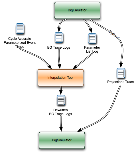
24 Flow diagram for use of the interpolation tool
1.4.1. Tool Usage
The interpolation tool is part of the regular Charm++ distribution and
can be found under the directory
charm/examples/bigsim/tools/rewritelog with a README file
describing its use in more detail than this manual.
1.4.1.1. Producing the Parameterized Timings Log
The interpolation tool uses as input a log of actual durations of user-bracketed sequential execution blocks. These timings come from a full or partial execution of the parallel application on a real machine or within a cycle-accurate simulator.
The user must insert startTraceBigSim() and endTraceBigSim()
calls around the main computational regions in the parallel application.
These two calls bracket the region of interest and print out a record
for that computational region. The functions should be called at most
once during any SEB. The output produced by endTraceBigSim() is a
line similar to
TRACEBIGSIM: event:{ PairCalculator::bwMultiplyHelper } time:{ 0.002586 } params:{ 16384.00 1.00 220.00 128.00 128.00 0.00 0.00 0.00 }.
The event name and the values (in double-precision floating-point) for
up to 20 parameters are specified in the call to endTraceBigSim();
the time field records the duration of the bracketed region of
sequential code.
To run in a cycle-accurate simulator such as IBM’s MAMBO, the
startTraceBigSim() and endTraceBigSim() functions would be
modified to switch between the “fast forward” mode used during the rest
of the program and the cycle-accurate mode during the bracketed region
of code. The functions are provided in C++ source files under the
directory charm/examples/bigsim/tools/rewritelog/traceBigSim and
their calls must be added to an application’s source file manually.
1.4.1.2. The BigSim log file format
To understand how the interpolation tool works, it is instructive to consider the format of logs produced by the BigSim Emulator. A BigSim log file (i.e. bgTrace log) contains data from emulation of the full parallel application. There is an entry for each SEB, with the following fields: ID, Name, \(T_{start}\), \(T_{end}\), Back, Forward, Message ID, Source Node, Message ID, Sent Messages. The final field is actually a list of records for each message sent by the execution block; each record contains the following fields: Message ID, \(T_{sent}\), \(T_{recv}\), Destination PE, Size, Group.
The interpolation tool will rewrite the durations of the SEBs by correcting the \(T_{end}\) field for the SEB and the \(T_{sent}\) fields for each message sent. The new durations of all SEBs will be based upon some model \(M:SEB\rightarrow Duration\).
Each SEB can be decomposed into three temporal regions as shown in
Figure 25:. The entire SEB is
associated with execution of a Charm++ entry method, while the middle
region is the computational kernel of interest, bracketed by the user’s
startTraceBigSim() and endTraceBigSim() calls. The model is used
only to approximate the new duration of the middle temporal region; the
durations of the beginning and ending regions are simply scaled by a
constant factor. Internally, the interpolation tool takes the ID for
each SEB and looks up its associated parameters. When those parameters
are found, they are used as input for evaluation of the new duration
\(d_{new}\) for the SEB. The end time is then modified to be
\(T_{end}\leftarrow T_{start}+d_{new}\).
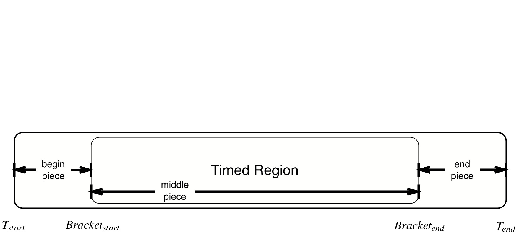
25 SEBs in the bgTrace file have a start and end time. Only a portion of the SEB, e.g. the important computational kernel, is timed when performing cycle accurate simulation. The duration of the middle portion of the SEB can be estimated in a different manner than the rest of the SEB. For example, the begin and end pieces can be scaled by some constant factor, while the bracketed middle region’s duration can be estimated based on a more sophisticated model.
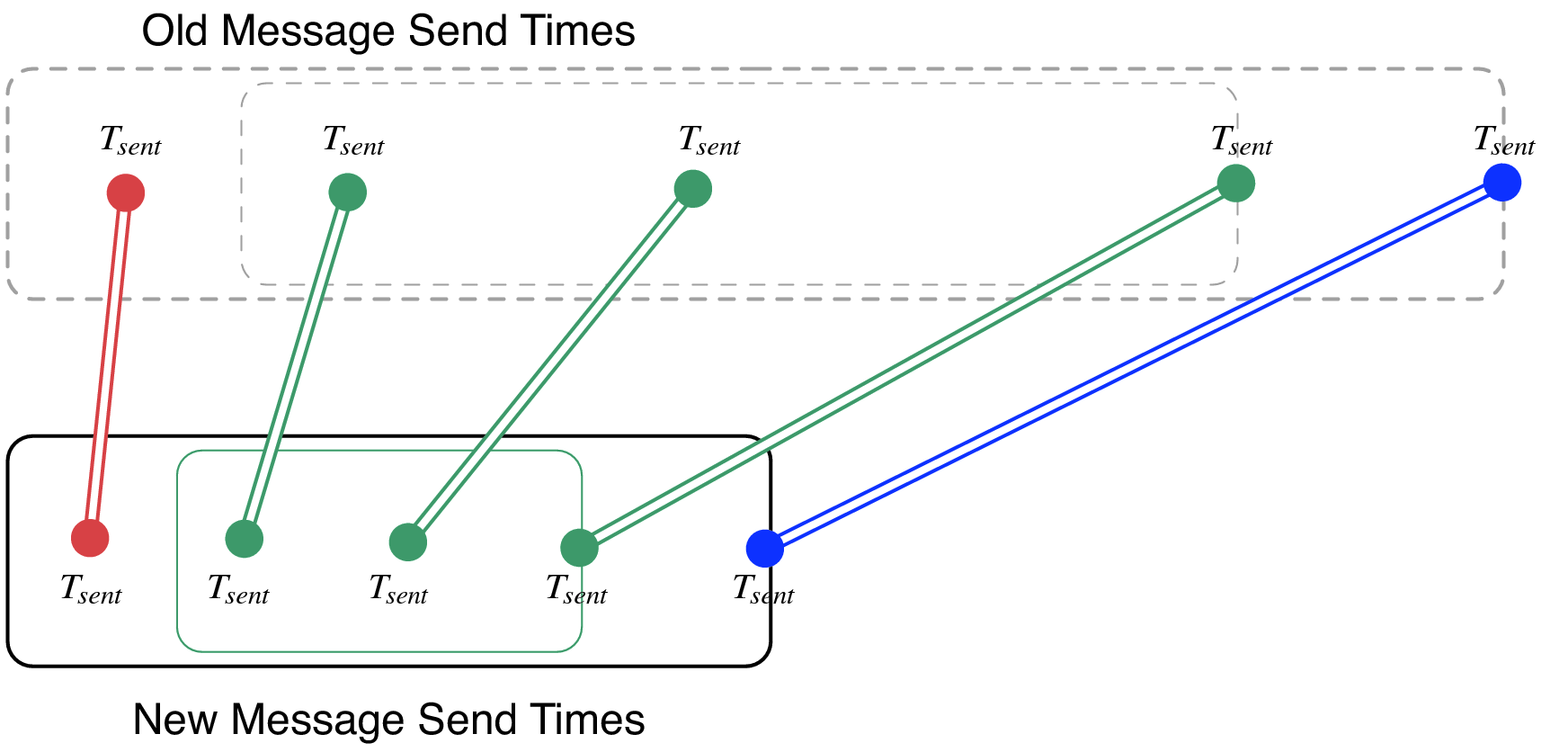
26 Message send times for messages sent from an SEB are remapped linearly onto the new time ranges for the SEB, region by region.
The messages in the message list for each SEB must also have their \(T_{sent}\) times rewritten. This is accomplished by linearly mapping the old \(T_{sent}\) value from to the new range for the enclosing SEB region, as shown in Figure 26. Any message sent during the first portion will be mapped linearly onto the new first portion of the SEB. The new message \(T_{recv}\) times are ignored by BigSimulator, so they do not need to be modified.
1.4.1.3. Supported performance models
The interpolation tool supports three types of models, as described in this subsection. The more sophisticated models use the least-square curve fitting technique. The current implementation uses the Gnu Scientific Library(gsl) to perform the least-square fit to the given data. The library provides both the coefficients and a \(\chi^2\) measure of the closeness of the fit to the input data.
1.4.1.3.1. Model 1: Scaling SEB durations by a constant factor
In simple cases, a sufficient approximation of the performance of a
parallel application can be obtained by simply scaling the SEB durations
by a constant factor. As an example, a user may know that a desired
target machine has processors that will execute each SEB twice as fast
as on an existing machine. The application is emulated on the existing
machine and the observed SEB durations are scaled by a factor of
\(2.0\). Although simple, this method may be sufficient in many
cases. It becomes unnecessary to use the startTraceBigSim() and
endTraceBigSim() calls. The scaling factor is hard coded in the
interpolation tool as time_dilation_factor. It is used to scale all
blocks unless a suitable advanced model has a better method for
approximating the block’s duration. It will always be used to scale any
portions of blocks that are not bracketed with the calls
startTraceBigSim() and endTraceBigSim().
1.4.1.3.2. Model 2: Extrapolation based on user’s parameterizations
The user can simply insert the bracketing calls startTraceBigSim()
and endTraceBigSim() around the computational kernels to log the
times taken for each kernel. In practice, the duration of the SEB will
likely depend upon the data distribution and access patterns for the
parallel application. Thus, the user must specify parameters likely to
influence the SEB duration. The parameters can include variables
indicating number of loop iterations, number of calls to computational
kernels, or sizes of accessed portions of data arrays. A model is built
to approximate the duration of any SEB based upon its specified
parameters.
As an example, NAMD uses a number of different types of objects. The
compute objects will spend varying amounts of time depending upon
the lengths of their associated atom lists. If an atom list is large,
more interactions are computed and thus more computation is performed.
Meanwhile, assume that a Charm++ entry method called
doWork(atomList) is where the majority of the work from an
application occurs. The function computes forces on atoms of various
types. Different calls to the function will contain different numbers
and types of atoms. The source code for doWork(atomList) will be
modified by the user to contain calls to startTraceBigSim() at the
entry and endTraceBigSim() at the exit of the function. The program
will be run, and the resulting timed samples will be used to build a
model. Assume the expected runtime of doWork(atomList) is quadratic
in the atomList length and linear in the number of carbon atoms in
the atomList. The endTraceBigSim() call would be provided with a
descriptive name and a set of parameters, such as
endTraceBigSim(“doWork()”, p_1,p_2), where parameter \(p_1\) is
the length of atomList and parameter \(p_2\) is the number of
carbon atoms in atomList.
The goal of using a model is to be able to predict the execution time of
any arbitrary call to doWork(), given its parameters. The
application can be run on an existing processor or parallel cluster for
only a few timesteps with the modified doWork() method. This run
will produce a list of
{\(\left(p_1,p_2\right)\rightarrow duration\)} records. A least
squares method is applied to fit a curve
\(f(p_1,p_2)=c_1+c_2 p_1+c_3 p_1^2 + c_4 p_2\) approximating the
durations of the records. The least square method minimizes the sum of
the squares of the difference between the function \(f\) evaluated
at each parameter set and the actual timing observed at those
parameters. The least square method is provided
\(\left(1.0,p_1,p_1^2,p_2,time\right)\) for each sample point and
produces the coefficients \(c_n\) in \(f\). An arbitrary set of
parameters (in the current implementation, up to twenty) can be input to
\(f\) to produce an approximation of the runtime of doWork()
even though the particular instance was never timed before.
1.4.1.3.3. Model 3: Extrapolation of partial executions with cycle accurate simulations and user’s parameterizations
In this case, a cycle accurate simulator can be used to simulate a small fraction of all SEBs for a run of the application. The partial execution is used to build a model which applies to the whole execution. Parameterizations can be used as previously described, so that only some fraction of the SEBs will be run in the expensive cycle-accurate simulator. In NAMD, for example, a sufficient model can be built from a random sample of 2% of the cycle-accurate SEB durations from four timeloop iterations.
1.5. BigSim Log Generation API
To be added …